Research: What do disc golf flight numbers actually mean? Explained with data.

Abstract: This is a short technical paper describing how we at HYZR ground flight numbers in real data. This is the process of turning the speed, glide, turn, fade and weight into real aerodynamic tables that are used in the simulation and accurately describe the flight characteristics of a disc.

The process consists of roughly three stages: A regression that uses a large library of physically scanned discs, blending the selected flight numbers with physical discs and fusing the result of these two to produce the aerodynamic properties of the disc.

The result is accuracy at the limit of what flight numbers can specify. The method also allows to use the fade as an input unlike traditional simplified methods better matching the players' expectations.

Motivation: In disc golf simulation, the "simulated" disc is arguably the largest source of error, bigger than sensor accuracy, physics model or environment factors. Especially on longer distance throws, small errors in the simulated disc accumulate and can poison the entire simulation.

For accurate results in the simulation, this is one of the most important problems to solve.

1. What we need to simulate a disc.

The simulation cannot directly consume the flight numbers, but rather aerodynamic tables (lift, drag and pitching moment), mass, diameter and two moments of inertia.

Mass, diameter and two moments of inertia can be measured from the physical disc + its 3D model. The aerodynamic tables are considerably more difficult. To obtain these, you can measure a disc in a wind tunnel, or use Computational Fluid Dynamics (CFD) which can be thought as a "virtual wind tunnel". This is the most time-consuming, expensive and sensitive part of the process.

Now, the problem is that all of the above requires the physical disc. For a custom disc we need a process that takes the flight numbers as an input and outputs a table that is plausible as a disc and best matches the intent of the user. Formally, this is:

G(s, g, t, f,m) → (CL[α], CD[α], CM[α], D, Ixy, Iz)

where CL, CD and CM are the lift, drag and pitching-moment curves as functions of the angle of attack (or more commonly "nose angle").

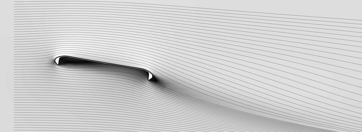
Figure 1: A visualization of Innova DX Aviar simulated in the CFD environment.

2. Notations

symbol	meaning
r = (s, g, t, f)	input flight numbers: speed, glide, turn, fade
u = −t	understability; turn is stamped negative, so this makes the sliders read upward
α	angle of attack ("nose angle"), degrees
F	the library of real discs measured in a wind tunnel or CFD
x̂ (hat)	a quantity predicted by the regressions
x̄ (bar)	the same quantity measured back off the blended carrier

Sign convention: C_M < 0 means the disc wants to turn over (RHBH), C_M > 0 means it wants to fade.

3. Stage 1: Regression

Identifying the key elements from a disc: Each wind tunnel measured or CFD simulated disc is compressed to N variables. These are the key data points from the disc that define how it flies and are used in the regression.

The most important one is the trim angle (T), which defines the AoA at which the CM crosses zero. A disc above its trim angle will fade and below it will turn.

Figure 2: A visualization of a pitching moment curve. The trim angle T is the angle of attack at which the CM crosses the zero line. In this example 3.2 degrees.

Regression: For each feature y, we design a matrix X whose columns are a constant and the flight numbers, (1, s, g, f, u), one row per disc in the library, and solve for the coefficient vector b:

min  ‖ X·b − y ‖²

For the example of the trim angle (T), we take the full library of the measured trim angles from the real discs and their reported flight numbers and regress to find the coefficients that minimize the error.

The result of the form: trim = b₀+b_s·speed + b_g ·glide + b_u·understability+ b_f·fade

Each coefficient tells us how much the reported flight number affects the trim angle of the disc.

This process is then repeated for each of the N variables used. 

4. Stage 2: The Blend

From the regressions, we have the properties that the created disc must have, but importantly not the real shape of a physical disc. Without this step, the result could be a table that no real disc could produce.

We get the shape from a Nadaraya-Watson average over the library of real measured discs in standardised rating space. Every disc contributes to the result and is weighted by how close it is to the requested disc.

The result of this computation is called "the carrier". The carrier has a set of curves that have the correct physical shape and is near the requested disc, but not exactly at it.

Because every disc contributes to the result, the model generalizes well and changes smoothly with the requested flight numbers. Even when we have an exact match to the flight numbers in the library, we don't use it directly. This guarantees that the variables such as brand, plastic and production are equally inherited by the result which leads to decreased errors.

As an example different 12,5,-1,3 discs fly very differently, depending on the brand, plastic, production run and more. Choosing one over the other would result in larger errors on average (see Figure 4).

Diameter and the two inertias ride the same weights.

5. Stage 3: Fusing

From above, we have the right shape, but the wrong properties. A disc near the request, but not right at it. As a next step, we fuse the results to obtain the final disc.

Essentially, the curves are adjusted to meet the requested variables, while still keeping the shape that grounds them in the physical discs. This is where many traditional simulators will fail and produce discs that are not physically feasible.

An example: Let a hat denote a regression target from stage 1 and a bar the same feature measured off the carrier. Let ΔT = T̂ − T̄. The issued moment curve is

v       =  CM(α − ΔT)
CM*(α)  =  v · (K̂ / K̄)     if v < 0
           v · (Q̂ / Q̄)     otherwise

where K is the depth of the turning branch and Q the slope of the fade branch.

For example: The blend gives us a trim of 2.57°, but the regressions ask for 3.19°. As a result, the moment curve is moved by 0.62° to meet the regression target. For reference on a distance throw, this moves the outcome by roughly 7 m / 23 ft.

Figure 3: Visualization of the trim example.

6. Accuracy and validation

The accuracy can be tested by leaving one real measured disc out and creating that disc with its flight numbers into the system and then comparing that flight to the output from the real measured disc.

This median on the worst case, a power throw that does a full s-turn, is ≈ 10m / 33ft and much less on pure hyzer or shorter throws.

Accuracy floor: Due to the flight numbers not being standardized, the error cannot be 0. We can prove this by running the same test with pairs of real measured discs with identical flight numbers. This gives us a median error of 17-18 m / ≈ 58 ft and the worst 57m / 187ft.

Figure 4: Example of six real discs with 12,5,-1,3 flight numbers. The discs have a large spread on an identical throw.

Our model beats matching requested discs to real ones by flight numbers directly. No numbers-only model can beat our method on average, even if it includes the fade as an input, because of the ambiguity.

7. Weaknesses

• The model is highly dependent on quality measured data from real discs which is difficult and expensive to obtain accurately. Coverage of the disc library is an important and ongoing work. Requested discs with no close references will have more error.
• The flight numbers are not yet standardized: Constant biases between brands, plastics and production runs are impossible to properly address, without having them as input data.
• Validation is done with other physical discs. The "real" error is the difference between the created disc and what the user intended which is difficult to measure.
  
• The CFD process has its own limitations that require additional stages, not described here.

8. Restricted data and access

Several of the steps are kept broad on purpose while others are completely left out. No real data is shared here and is kept private for now.

However, this gives enough information to evaluate and build upon our work.

The full data is available for academic research use. Contact us for access.

HYZR - 08/2026 - gethyzr.com